The source code of this project is hosted on my WDClassification Github repository.

About

This project is an example applying machine-learning algorithms and pure data science to a topic in astrophysics. In the study of white dwarfs (WDs), there have been distinct subclasses of these stars that have been found, each with different physical features. These classes can be summarized by the following:

Class	Spectroscopic features
DA	H
DB	He I
DC	Continuous spectrum
DO	He II with He I or H
DZ	Metal lines
DQ	Carbon lines
DX	Unclassified

Classifications in many topics in astrophysics play a cruicial role in the comparison with physical models in order to understand the diversity of these astronomical object and to understand the physical mechanisms governing their evolution and existence. Therefore, creating a classification model for these objects, including white dwarfs, is a very beneficial scientific tool.

Results: Montreal WD Database (MWDD)

MWDD contains data of around 40,000 white dwarfs, including their physical parameters such as effective temperature (T_eff), mass, and log(g), and other observed quantities such as photometry. Importantly, MWDD also contains the spectral class (DA, DB, etc.) for each of these white dwarfs. In this project, we make use of some of these physical parameters along with SDSS photometry (ugriz bands) to develop a classification model for these white dwarfs. It would be very advantageous to be able to classify a spectroscopic subtype of a white dwarf given mostly just its observed photometry, as it is generally easier to obtain more numerous and accurate photometric observations of objects than their spectroscopy.

This project is carried out using Python JupyterLab notebooks (using scikit-learn), which can be found in my Github repo mentioned at the top of this page. Here, we summarize the data science process and some of the main results.

Data Selection

See the preprocessing notebook for the specifics on preprocessing this data.

Some of the main points leading to training the models:

• We choose not to do imputation of missing values, as the underlying distribution of features is unknown, and the sample size is big enough to not worry.
• After removing samples with missing T_eff, mass, log(g), and photometry, a sample size of N = 30,688 remains.
• Colors (g-r, r-i, etc.) were also calculated and provided to the model.
• It turns out that DA WDs make up about 80% of the sample, so we choose to make models that classify DAs versus non-DAs, and separate models are made to distinguish other classes.
• To not overwhelm the models that classify DAs and non-DAs with a vast majority of DA objects, removing a large fraction (~60%!) of DAs from the sample greatly improves models. This fraction was chosen to optimize the performance of the models. N = 14,430 total WDs are leftover to train the the model that distinguishes non-DAs from DAs.
• N = 4,810 non-DA WDs are available to train the secondary model for other classes.

Model Results

See the modeling notebook for the specifics on the models tested and their evaluations.

Here we tested multiple classification models: Random forest (RF), Gradient boosting (GB), and K-nearest neighbors (KNN). 80% of the sample was used to train each model, and the remaining 20% was used for model evaluation. We did a cross-validation grid search on each of these to determine good parameters to use for each. The model was then evaluated in performance; the results of each are summarized below:

Random Forest:

Merit	|	DA	non-DA	|	DB	DC	DQ	DZ	DO
Precision	|	0.890	0.911	|	0.937	0.747	0.800	0.759	0.769
Recall	|	0.808	0.952	|	0.980	0.887	0.941	0.526	0.470

Gradient-Boosting:

Merit	|	DA	non-DA	|	DB	DC	DQ	DZ	DO
Precision	|	0.882	0.921	|	0.958	0.830	0.800	0.785	0.806
Recall	|	0.831	0.947	|	0.977	0.899	0.941	0.654	0.671

K-Nearest Neighbors:

Merit	|	DA	non-DA	|	DB	DC	DQ	DZ	DO
Precision	|	0.760	0.870	|	0.896	0.691	1.000	0.735	0.718
Recall	|	0.724	0.890	|	0.972	0.822	0.882	0.462	0.409

The model that performed best overall and most consistently, especially in distinguishing between non-DA WDs, was the gradient-boosting model. A visual representation of its performance is shown below as confusion matrices:

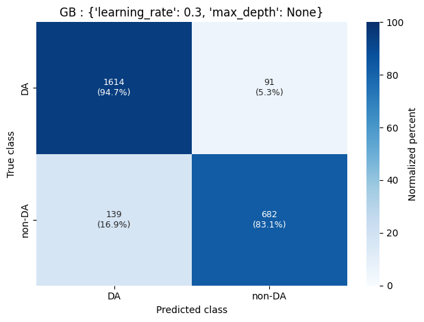Confusion matrix of gradient-boosting algorithm classifying DA and non-DA WDs.

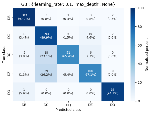Confusion matrix of gradient-boosting algorithm classifying non-DA WDs.

These results are very similar and sometimes improved from those by García-Zamora, et al. (2023) who used Random Forests with a set of 110 spectral coefficients to determine the same classification scheme.

The Random Forest method also performs similarly to the Gradient-Boosting method; however, it heavily struggles in classifying DZ objects. Perhaps with a higher number of estimators available to the RF model, this can be mitigated. Unfortunately, training the RF model is already much more computationally intensive (it took ~10x longer to train on a single processor for similarly sized parameter grids), so this is another case of trade-off between accuracy and time/resources.

Feature Importance from Random Forest

Although the Random Forest procedure does not produce the best results in this work, it is still beneficial as it allows for a convenient way of looking at the importance of the features provided to train the model. For example, we can look at the impurity-based feature importances given by the RF model:

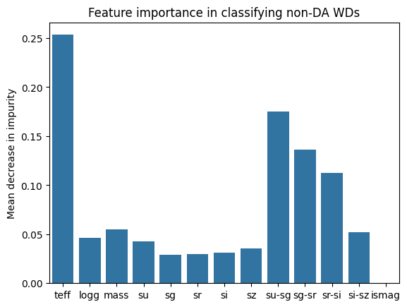Most importance features deemed by the Random Forest model.

The important features are similar for the model distinguishing between DAs and non-DAs. In this example, we see that u-g and effective temperature play a large role in objects being classified as one class or another.